Purpose
The purpose of this post is to investigate how to process in parallel sources extracted from full sky maps, in this case the maps release by Planck, using Hadoop instead of more traditional MPI-based HPC custom software.
Hadoop is the MapReduce implementation most used in the enterprise world and it has been traditionally used to process huge amount of text data (~ TBs) , e.g. web pages or logs, over thousands commodity computers connected over ethernet.
It allows to distribute the data across the nodes on a distributed file-system (HDFS) and then analyze them (“map” step) locally on each node, the output of the map step is traditionally a set of text (key, value) pairs, that are then sorted by the framework and passed to the “reduce” algorithm, which typically aggregates them and then save them to the distributed file-system.
Hadoop gives robustness to this process by rerunning failed jobs, distribute the data with redundancy and re-distribute in case of failures, among many other features.
Most scientist use HPC supercomputers for running large data processing software. Using HPC is necessary for algorithms that require frequent communication across the nodes, implemented via MPI calls over a dedicated high speed network (e.g. infiniband). However, often HPC resources are used for running a large number of jobs that are loosely coupled, i.e. each job runs mostly independently of the others, just a sort of aggregation is performed at the end. In this cases the use of a robust and flexible framework like Hadoop could be beneficial.
Problem description
The Planck collaboration (btw I’m part of it…) released in May 2013 a set of full sky maps in Temperature at 9 different frequencies and catalogs of point and extended galactic and extragalactic sources:
Each catalog contains about 1000 sources, and the collaboration released the location and flux of each source.
The purpose of the analysis is to read each of the sky maps, slice out the section of the map around each source and perform some analysis on that patch of sky, as a simple example, to test the infrastructure, I am just going to compute the mean of the pixels located 10 arcminutes around the center of each source.
In a production run, we might for example run aperture photometry on each source, or fitting for the source center to check for pointing accuracy.
Sources
All files are available on github:Hadoop setup
I am running on the San Diego Supercomputing data intensive cluster Gordon:
Note: Gordon has been retired. See SDSC for current resources.
SDSC had a simplified Hadoop setup based on shell scripts, myHadoop, which allowed running Hadoop as a regular PBS job.
The most interesting feature was that the Hadoop distributed file-system HDFS was setup on the low-latency local flash drives, one of the distinctive features of Gordon.
Using Python with Hadoop-streaming
Hadoop applications run natively in Java, however thanks to Hadoop-streaming, we can use stdin and stdout to communicate with a script implemented in any programming language.
One of the most common choices for scientific applications is Python.
Application design
Best way to decrease the coupling between different parallel jobs for this application is, instead of analyzing one source at a time, analyze a patch of sky at a time, and loop through all the sources in that region.
Therefore the largest amount data, the sky map, is only read once by a process, and all the sources are processed. I pre-process the sky map by splitting it in 10x10 degrees patches, saving a 2 columns array with pixel index and map temperature ( preprocessing.py ).
Of course this will produce jobs whose length might be very different, due to the different effective sky area at poles and at equator, and by random number of source per patch, but that’s something we do not worry about, that is exactly what Hadoop takes care of.
Implementation
Input data
The pre-processed patches of sky are available in binary format on a lustre file-system shared by the processes.
Therefore the text input files for the hadoop jobs are just the list of filenames of the sky patches, one per row.
Mapper
The mapper is fed by Hadoop via stdin with a number of lines extracted from the input files and returns a (key, value) text output for each source and for each statistics we compute on the source.
In this simple scenario, the only returned key printed to stdout is “SOURCENAME_10arcminmean”.
For example, we can run a serial test by running:
and the returned output is:
Reducer
There is no need for a reducer in this scenario, so Hadoop will just use the default IdentityReducer, which just aggregates all the mappers outputs to a single output file.
Hadoop call
The hadoop call is:
$HADOOP_HOME/bin/hadoop –config $HADOOP_CONF_DIR jar $HADOOP_HOME/contrib/streaming/hadoopstreaming.jar -file $FOLDER/mapper.py -mapper \(FOLDER/mapper.py -input /user/\)USER/Input/* -output /user/$USER/Output
So we are using the Hadoop-streaming interface and providing just the mapper, the input text files (list of sources) had been already copied to HDFS, the output needs then to be copied from HDFS to the local file-system, see run.pbs.
Hadoop run and results
For testing purposes we have just used 2 of the 9 maps (30 and 70 GHz), and processed all the total of ~2000 sources running Hadoop on 4 nodes.
Processing takes about 5 minutes, Hadoop automatically chooses the number of mappers, and in this case only uses 2 mappers, as I think it reserves a couple of nodes to run the Scheduler and auxiliary processes.
The outputs of the mappers are then joined, sorted and written on a single file, see the output file
See the full log sample_logs.txt extracted running:
/opt/hadoop/bin/hadoop job -history output
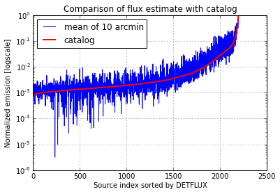
Comparison of the results with the catalog
Just for a rough consistency check, I compared the normalized temperatures computed with Hadoop using just the mean of the pixels in a radius of 10 arcmin to the fluxes computed by the Planck collaboration. I find a general agreement with the expected noise excess.