import healpy as hp
import numpy as np
import astropy.units as u
hp.disable_warnings()If you are analyzing a map from an instrument with a specific beam width, you can correct the power spectrum by the smoothing factor caused by that beam and obtain a better approximation of the power spectrum of the orignal sky.
m, h = hp.read_map(
    "https://portal.nersc.gov/project/cmb/so_pysm_models_data/equatorial/dust_T_ns512.fits", h=True
)
hp.mollview(m, min=0, max=1000, title="Dust map", unit="uK_RJ")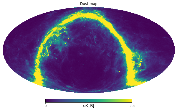
cl = hp.anafast(m)In this case we assume that the dust map from PySM is the true sky, then we apply a smoothing caused by the beam
beam = 30 * u.arcminm_smoothed = hp.smoothing(m, fwhm=beam.to_value(u.radian))cl_smoothed = hp.anafast(m_smoothed)We can get the transfer function of the beam, generally referred as \(B_\ell\):
bl = hp.gauss_beam(fwhm=beam.to_value(u.radian), lmax=len(cl)-1)import matplotlib.pyplot as pltplt.loglog(bl)
plt.title("Beam window function")
plt.xlabel("$\ell$");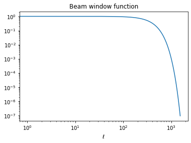
hp.mollview(m_smoothed, min=0, max=1000)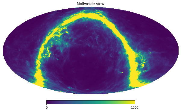
We can recover the input \(C_\ell\) as $C_^{input} = $:
plt.style.use("seaborn-talk")
plt.loglog(cl, label="cl")
plt.plot(cl_smoothed, label="cl smoothed")
plt.plot(cl_smoothed/bl**2, label="cl smoothed corrected")
plt.xlim(1, len(cl)+100)
plt.axvline(1100, color="gray", ls="--", label="$\ell=1100$");
plt.legend()
plt.grid();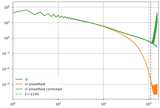
However, once the smoothed \(C_\ell\) reach machine precision, there is no more signal left, the beam deconvolution then causes extra noise. We need to limit our analysis to a range of \(\ell\) before the numerical error dominates, in this case for example, \(\ell=1100\).