Why 3 pixels per beam? The mathematics of HEALPix resolution matching
Exploring why the Planck convention uses FWHM = 3 x pixel size for harmonic-space map downgrading, with equations from the literature and simulated demonstrations.
Why 3 Pixels Per Beam? The Mathematics of HEALPix Resolution Matching
When downgrading HEALPix maps in harmonic space, the standard practice is to smooth the output map with a Gaussian beam whose FWHM is approximately 3 times the pixel size. This convention has roots in general radio and optical astronomy sampling theory (Robertson 2017) and was codified for CMB analysis by the Planck collaboration. This notebook explores why this factor of 3 works, tracing the reasoning through sampling theory, the HEALPix pixel window function, and anti-aliasing requirements. We demonstrate each concept with simulated maps.
import numpy as npimport healpy as hpimport matplotlib.pyplot as plt%matplotlib inlineplt.rcParams.update({"figure.dpi": 120, "font.size": 11})# Planck 2013 XXIII Table 1: FWHM = 160 arcmin at Nside=64, giving ratio 2.91# This is the exact scaling used consistently across all Planck resolutions.PLANCK_K =160.0/ (np.degrees(hp.nside2resol(64)) *60)print(f"healpy {hp.__version__}, numpy {np.__version__}")print(f"Planck FWHM/pixel ratio: {PLANCK_K:.4f}")
2. HEALPix Basics: Pixels, Bandlimits, and the Pixel Window
2.1 Pixel size
A HEALPix grid at resolution parameter \(N_{\mathrm{side}}\) divides the sphere into \(N_{\mathrm{pix}} = 12 \, N_{\mathrm{side}}^2\) equal-area pixels. The characteristic pixel size is (Górski et al. 2005, Eq. 2):
The standard HEALPix bandlimit is \(\ell_{\max} = 3 \, N_{\mathrm{side}} - 1\). This is not a Nyquist limit — it is the maximum multipole for which the SHT quadrature weights converge well. With pixel weights, exact recovery is possible up to \(\ell_{\max} = 1.5 \, N_{\mathrm{side}}\) (healpy issue #356).
2.3 Pixel window function
Each HEALPix pixel averages the sky signal over a finite area. This averaging acts as a convolution, described in harmonic space by the pixel window function\(p_\ell\) (Górski et al. 2005, §5.2). Sullivan et al. (2024), Eq. 15, provide the approximate form:
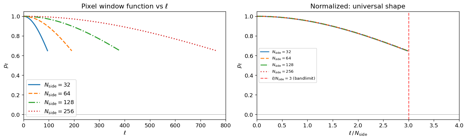
Let’s compute and plot the exact pixel window functions for several \(N_{\mathrm{side}}\) values. When we normalize \(\ell\) by \(N_{\mathrm{side}}\), the pixel windows for different resolutions nearly overlap — this is the universal shape of the HEALPix pixel averaging kernel. We plot them at their native \(\ell\) range to see the differences.
  p_{ell} at ell = 1.5 * Nside = 96: 0.8986
  p_{ell} at ell = 2.0 * Nside = 128: 0.8261
  p_{ell} at ell = 3*Nside-1 = 191: 0.6479
What we see: The left panel shows the pixel window function \(p_\ell\) for four different resolutions, each plotted against its native multipole \(\ell\) with distinct colors and linestyles. Higher \(N_{\mathrm{side}}\) means finer pixels, so the window extends to higher \(\ell\) before dropping — each resolution has a bandlimit of \(3N_{\mathrm{side}}-1\). The right panel rescales the x-axis to \(\ell / N_{\mathrm{side}}\): all four curves collapse onto a single universal shape, confirming that pixel averaging has the same relative effect at every resolution. The pixel window at the bandlimit \(\ell = 3N_{\mathrm{side}}\) (red dashed line) is always \(\approx 0.65\), meaning the pixels already attenuate high-\(\ell\) power by ~35% even before any smoothing beam is applied. This inherent attenuation contributes to the combined suppression studied in Section 4.
3. The Planck Equation: Harmonic-Space Resolution Change
Planck 2013 XXIII, Table 1: The 3-pixel rule in practice
Planck 2013 XXIII lists the masks used for CMB analysis at each resolution. Each mask is produced by degrading a high-resolution mask to a lower \(N_{\mathrm{side}}\), and the smoothing beam is chosen as FWHM = 3 × pixel size — consistently across all eight resolutions. The table below reproduces the Nside/FWHM columns and adds the computed pixel size and FWHM/pixel ratio to make this explicit.
What we see: The ratio FWHM / pixel size is exactly 2.91 at every resolution — not precisely 3. This is because Planck uses FWHM = 160 arcmin × (64 / \(N_{\mathrm{side}}\)), while the HEALPix pixel size scales as \(\theta_{\mathrm{pix}} \approx 3517 / N_{\mathrm{side}}\) arcmin, giving a fixed ratio of \(160 \times 64 / 3517 \approx 2.91\). The “3 pixels per beam” label is a rounded description of this convention. The constant ratio across all eight resolutions confirms that a single rule was applied uniformly, and that the choice was deliberate rather than resolution-specific tuning.
4. Why ~3? Sampling Theory on the Sphere
4.1 The Nyquist analogy (and its limits)
In 1D, the Nyquist–Shannon theorem requires \(\geq 2\) samples per wavelength. On the sphere, multipole \(\ell\) corresponds to an angular wavelength \(\lambda_\ell \approx 2\pi / \ell\). At the HEALPix bandlimit \(\ell_{\max} = 3 N_{\mathrm{side}} - 1\):
So there are about 2 pixels per wavelength at the bandlimit — right at the Nyquist rate. This is marginal: any power above the bandlimit will alias.
4.2 The beam as an anti-aliasing filter
The role of the output beam \(b^{\mathrm{out}}_\ell\) is to act as a low-pass (anti-aliasing) filter, suppressing power near and above \(\ell_{\max}\) before the signal is discretized onto the output pixel grid.
A Gaussian beam with \(\mathrm{FWHM} = k \times \theta_{\mathrm{pix}}\) attenuates multipole \(\ell\) by:
Let’s evaluate this for different \(k\) (using \(3\pi / (16 \ln 2) \approx 0.850\)):
\(k\) (FWHM / pixel)
\(b_{\ell_{\max}}\) (approx.)
Amplitude suppression
1
0.428
57% — substantial aliasing leakage
2
0.033
97% — good, but near-bandlimit power is only partly attenuated
2.91 (Planck)
~0.00075
>99.9% — near-perfect anti-aliasing
3 (nominal)
~0.00048
>99.9% — similar, slightly more aggressive
4
1.2×10⁻⁶
≈100% — negligible further improvement
At \(k = 2.91\) (the actual Planck ratio), the beam amplitude at the bandlimit is \(\approx 0.00075\) — effectively zero. The difference between \(k=2.91\) and the rounded value \(k=3\) is negligible in practice (\(b_\ell\) changes by a factor of ~1.6 between them, but both are already vanishingly small). This is the sweet spot:
\(k = 1\): 57% amplitude suppression → heavy aliasing from near-bandlimit power
\(k = 2\): 97% suppression at \(\ell_{\max}\), but the attenuation is gradual — power at intermediate \(\ell \sim 0.5\,\ell_{\max}\) is only reduced by ~60%, so aliasing from a broad range below the bandlimit can still accumulate
\(k \approx 2.91\) (Planck): >99.9% suppression at \(\ell_{\max}\) and strong attenuation throughout the high-\(\ell\) range — the law of diminishing returns begins here
\(k = 4\): negligible improvement over \(k \approx 2.91\) with unnecessary loss of angular resolution
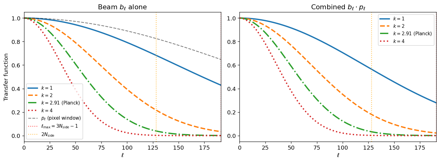
4.3 Combined beam × pixel window suppression
The total transfer function applied to the output map is \(b_\ell \cdot p_\ell\). Even where the beam alone isn’t fully suppressive, the pixel window provides additional attenuation. Let’s verify this numerically.
What we see: The left panel shows the Gaussian beam transfer function \(b_\ell\) for each \(k\) (distinct colors and linestyles). At \(k=1\), the beam still transmits ~43% of the signal amplitude at the bandlimit \(\ell_{\max}\) — well short of effective anti-aliasing. At \(k=2\), the drop reaches ~3%. At the Planck ratio \(k=2.91\), the beam is essentially zero (\(\approx 0.00075\)) at the bandlimit, providing near-perfect suppression. The dashed black curve is the pixel window \(p_\ell\) for reference.
The right panel shows the combined effect \(b_\ell \cdot p_\ell\) — the total attenuation seen by the output map. At \(k=2.91\), the combined transfer function is negligible above \(\ell \approx 140\) (for \(N_{\mathrm{side}}=64\)), making aliasing essentially impossible. At \(k=1\) or \(k=2\), significant power survives near the bandlimit and would alias back into lower multipoles when the alm are synthesized onto the coarser grid.
5. Demo 1: Beam Transfer Functions — Where Does Each \(k\) Cut Off?
Let’s quantify the effective bandwidth preserved by each beam choice. We define the “effective \(\ell_{\max}\)” as the multipole where \(b_\ell\) drops to 50%.
nside_out =64theta_pix = hp.nside2resol(nside_out)bandlimit =3* nside_out -1print(f"Nside_out = {nside_out}, theta_pix = {np.degrees(theta_pix)*60:.1f} arcmin, bandlimit = {bandlimit}")print(f"{'k':>6s}{'FWHM (arcmin)':>14s}{'ell at b_l=0.5':>15s}{'ell at b_l=0.1':>15s}{'fraction of bandlimit at 50%':>30s}")for k in [1, 2, PLANCK_K, 4]: fwhm = k * theta_pix bl = hp.gauss_beam(fwhm, lmax=bandlimit) ell50 = np.argmin(np.abs(bl -0.5)) ell10 = np.argmin(np.abs(bl -0.1)) tag =" (Planck)"if k == PLANCK_K else""print(f"{k:>6.2f}{np.degrees(fwhm)*60:>14.1f}{ell50:>15d}{ell10:>15d}{ell50/bandlimit:>30.1%}{tag}")
Nside_out = 64, theta_pix = 55.0 arcmin, bandlimit = 191
     k   FWHM (arcmin)   ell at b_l=0.5   ell at b_l=0.1    fraction of bandlimit at 50%
  1.00            55.0              173              191                           90.6%
  2.00           109.9               86              158                           45.0%
  2.91           160.0               59              108                           30.9% (Planck)
  4.00           219.9               43               79                           22.5%
What we see: The table quantifies the resolution–aliasing trade-off for \(N_{\mathrm{side}}=64\) (\(\ell_{\max}=191\)). At \(k=1\), the half-power point (\(b_\ell = 0.5\)) is reached at \(\ell \approx 173\) — almost the entire band is preserved, but at the cost of heavy aliasing. At the Planck ratio \(k=2.91\), the half-power point falls at \(\ell \approx 58\) (about 30% of the bandlimit): roughly the lower third of multipoles are well-preserved, the middle third are partially attenuated, and the upper third are strongly suppressed. This is the deliberate trade: sacrifice the highest multipoles (most prone to aliasing) to protect the lower ones. At \(k=4\), the half-power point drops to ~22% of the bandlimit — too aggressive, unnecessarily discarding well-resolved structure.
6. Demo 2: Anti-Aliasing — Downgrading a Known-Spectrum Map
We generate a map at high resolution with a known \(C_\ell\) (CMB-like power spectrum), downgrade it to low resolution with different beam choices, and measure the aliasing artifact in the power spectrum.
The input spectrum is a simple power law \(C_\ell \propto \ell^{-2}\) (roughly CMB-like), extending to \(\ell_{\max}^{\mathrm{in}}\).
Unable to display output for mime type(s): application/vnd.plotly.v1+json
What we see: We generated a map at \(N_{\mathrm{side}}=256\) with a power-law spectrum \(C_\ell \propto \ell^{-2}\) and downgraded it to \(N_{\mathrm{side}}=64\) using five harmonic methods (plus ud_grade). The Planck curve at \(k=2.91\) (thick red solid) uses the exact ratio from Planck 2013 XXIII Table 1.
ud_grade excess at high \(\ell\):ud_grade simply averages sub-pixels in real space — it does not bandlimit the input first. Modes from the full input grid (up to \(\ell_{\max}^{\mathrm{in}} = 3 \times 256 - 1 = 767\)) are all folded into the coarser output pixels. In harmonic space this is aliasing: input modes between \(\ell_{\max}^{\mathrm{out}} = 191\) and \(767\) alias back into lower multipoles. When we then divide the output spectrum by \(p_\ell^{\mathrm{out}\,2}\) to estimate the underlying spectrum, those aliased contributions appear as a large excess at high \(\ell\). There is no beam to suppress them before the averaging occurs.
Left panel: All harmonic spectra are deconvolved — divided by \(b_\ell^2 \cdot p_\ell^2\) — to estimate the underlying spectrum. A perfect downgrade recovers the black input curve. The \(k=0\) curve (purple, plotted on top) traces the truth almost exactly: for this smooth, bandlimited input there is no aliasing, so applying no beam with pure pixel-window correction is nearly lossless. In practice, real maps contain noise and sub-pixel structure that would cause \(k=0\) to diverge at high \(\ell\) for the same reason as ud_grade. Higher \(k\) values progressively suppress the high-\(\ell\) modes.
Right panel:\(k=1\) and \(k=2\) have the smallest fractional errors for this smooth test case — they filter the least and the input has no aliased power to suppress. This does not mean they are optimal in practice: real sky observations contain noise and systematics concentrated at high \(\ell\), where modes near \(\ell_{\max}\) are unreliable. The Planck \(k=2.91\) is a conservative safety margin that explicitly suppresses all modes beyond \(\ell \approx 60\) (about 30% of the bandlimit), trading some high-\(\ell\) fidelity for robust aliasing protection. Any upturn visible for \(k=2.91\) and \(k=4\) above \(\ell \sim 160\) is deconvolution noise (dividing by a near-zero transfer function), not real signal loss.
7. Demo 3: Noise Aliasing — Why Small \(k\) Fails in Practice
Demo 2 used a smooth, bandlimited input map with no noise. In that ideal case \(k=0\) and \(k=1\) look fine — there is simply nothing to alias. Real observations contain pixel-level noise (detector noise, CMB foreground residuals, sub-pixel signal) with power distributed up to the full input bandlimit \(\ell_{\max}^{\mathrm{in}}\). This demo repeats the downgrade with signal + white noise and directly measures how much noise leaks into the output map for each \(k\).
import plotly.graph_objects as gofrom plotly.subplots import make_subplots# Same parameters as Demo 2nside_in =256nside_out =64lmax_out =3* nside_out -1lmax_in =3* nside_in -1np.random.seed(42)theta_pix_out = hp.nside2resol(nside_out)pw_in_2b = hp.pixwin(nside_in)[:lmax_out +1]pw_out_2b = hp.pixwin(nside_out)[:lmax_out +1]ell_in_2b = np.arange(lmax_in +1, dtype=float)ell_out_2b = np.arange(lmax_out +1)# Signal: same C_ℓ ~ ℓ^{-2} as Demo 2cl_signal_2b = np.zeros(lmax_in +1)cl_signal_2b[2:] =1.0/ ell_in_2b[2:] **2signal_map_2b = hp.synfast(cl_signal_2b, nside_in, lmax=lmax_in, new=True)# White noise: flat C_ℓ equal to signal at ℓ_knee → noise dominates above ℓ_kneeell_knee =50cl_white_2b = np.zeros(lmax_in +1)cl_white_2b[2:] = cl_signal_2b[ell_knee] # = 1/50^2 = 4e-4 (flat)noise_map_2b = hp.synfast(cl_white_2b, nside_in, lmax=lmax_in, new=True)noisy_map_2b = signal_map_2b + noise_map_2b# Downgrade both signal-only and noisy maps with each kk_list_2b = [0, 1, 2, PLANCK_K, 4]clean_2b = {}noisy_2b = {}for k in k_list_2b:for src, dst in [(signal_map_2b, clean_2b), (noisy_map_2b, noisy_2b)]: alm = hp.map2alm(src, lmax=lmax_out, use_pixel_weights=True) bl = hp.gauss_beam(k * theta_pix_out, lmax=lmax_out) if k >0else np.ones(lmax_out +1) dst[k] = hp.alm2map(hp.almxfl(alm, (pw_out_2b / pw_in_2b) * bl), nside_out)# ud_grade: pixel-space averaging (no beam, no bandlimiting)ud_clean_2b = hp.ud_grade(signal_map_2b, nside_out)ud_noisy_2b = hp.ud_grade(noisy_map_2b, nside_out)cl_noise_ud_2b = hp.anafast(ud_noisy_2b - ud_clean_2b, lmax=lmax_out)# Noise contamination = noisy output - clean output (isolates noise contribution exactly)cl_noise_2b = {k: hp.anafast(noisy_2b[k] - clean_2b[k], lmax=lmax_out) for k in k_list_2b}cl_sig_ref_2b = cl_signal_2b[:lmax_out +1]k_styles_2b = [ (0, "#9467bd", "longdashdot", 2.5, "No beam (k=0)"), (1, "#ff7f0e", "dash", 1.5, "k=1"), (2, "#2ca02c", "dashdot", 1.5, "k=2"), (PLANCK_K, "red", "solid", 3.0, f"k={PLANCK_K:.2f} (Planck)"), (4, "#d62728", "dot", 1.5, "k=4"),]fig = make_subplots(rows=1, cols=2, subplot_titles=("Noise contamination in output","Noise-to-signal ratio in output"), horizontal_spacing=0.1)ell_x = ell_out_2b[2:]# ud_grade traces (both panels)fig.add_trace(go.Scatter(x=ell_x, y=cl_noise_ud_2b[2:], name="ud_grade", line=dict(color="gray", width=2, dash="longdash"), legendgroup="ud_grade"), row=1, col=1)fig.add_trace(go.Scatter(x=ell_x, y=cl_noise_ud_2b[2:] / cl_sig_ref_2b[2:], name="ud_grade", line=dict(color="gray", width=2, dash="longdash"), legendgroup="ud_grade", showlegend=False), row=1, col=2)for k, color, dash, lw, lbl in k_styles_2b: fig.add_trace(go.Scatter(x=ell_x, y=cl_noise_2b[k][2:], name=lbl, line=dict(color=color, width=lw, dash=dash), legendgroup=lbl), row=1, col=1) nsr = cl_noise_2b[k][2:] / cl_sig_ref_2b[2:] fig.add_trace(go.Scatter(x=ell_x, y=nsr, name=lbl, line=dict(color=color, width=lw, dash=dash), legendgroup=lbl, showlegend=False), row=1, col=2)fig.add_trace(go.Scatter(x=ell_x, y=cl_sig_ref_2b[2:], name="Signal C_ℓ (reference)", line=dict(color="black", width=2), opacity=0.5, legendgroup="signal"), row=1, col=1)# y=1 reference line on right panel (noise = signal)fig.add_hline(y=1.0, line=dict(color="black", width=1.5, dash="dot"), row=1, col=2)fig.add_trace(go.Scatter(x=[None], y=[None], name="noise = signal (y=1)", line=dict(color="black", width=1.5, dash="dot"), legendgroup="ref"), row=1, col=2)fig.update_xaxes(title_text="ℓ")fig.update_yaxes(type="log", title_text="C_ℓ (noise in output)", row=1, col=1)fig.update_yaxes(type="log", title_text="Noise C_ℓ / Signal C_ℓ", row=1, col=2)fig.update_layout(height=480, legend=dict(groupclick="togglegroup"))fig.show()
Unable to display output for mime type(s): application/vnd.plotly.v1+json
What we see: We added white noise (flat \(C_\ell^{\rm noise} = {\rm const}\), equal to the signal at \(\ell=50\), so noise dominates signal at \(\ell > 50\)) to the same \(N_{\rm side}=256\) input map, then downgraded to \(N_{\rm side}=64\) with each \(k\) and with ud_grade.
Left panel:\(C_\ell\) of the noise contamination in the output — isolated by subtracting the signal-only downgrade from the noisy downgrade — alongside the reference signal \(C_\ell\) (black). For \(k=0\) (no beam), the noise passes through nearly unchanged: the contamination equals or exceeds the signal across essentially the entire band. ud_grade behaves similarly — it performs real-space averaging with no beam suppression, so broadband noise aliases freely into the output. For \(k=1\), the beam only weakly suppresses noise (\(b_\ell \approx 0.43\) at \(\ell_{\max}\)), so contamination still dominates at high \(\ell\). At \(k=2.91\) (Planck), the noise contamination falls well below the signal at all multipoles — the beam has filtered out the aliasable noise before it can corrupt the output.
Right panel: Noise-to-signal ratio. Above the black dotted line (\(= 1\)), noise contamination exceeds signal — the output is unreliable. For \(k=0\), \(k=1\), and ud_grade, the ratio climbs steeply above 1 past \(\ell \approx 50\): the entire upper half of the output band is noise-dominated. This is exactly the failure mode that was invisible in Demo 2’s smooth, noiseless test. For \(k=2.91\), the ratio stays well below 1 across the full band — the motivation for Planck’s choice is clear: even with significant pixel noise, no multipole of the output map is corrupted by noise aliasing.
8. Demo 4: Power Spectrum Recovery — Quantitative Comparison
Let’s compute a single metric: the RMS fractional error in \(C_\ell\) over the “safe” multipole range \(2 \leq \ell \leq 2 N_{\mathrm{side,out}}\) (the conservative bandlimit).
What we see: Over the conservative multipole range \(\ell \leq 2 N_{\mathrm{side}}\), all harmonic methods achieve low RMS errors and substantially outperform ud_grade. This is because ud_grade uses simple pixel-space averaging and does not correct for the pixel window function, so even at low \(\ell\) it carries a systematic bias. Among the harmonic methods, differences are small in this safe range because aliasing mostly affects the highest multipoles near the bandlimit. The benefit of \(k=3\) over \(k=0\) or \(k=1\) becomes clear when the multipole range is extended toward \(\ell_{\max}\): the beam suppresses the near-bandlimit power that would otherwise alias, keeping the error bounded across the full band.
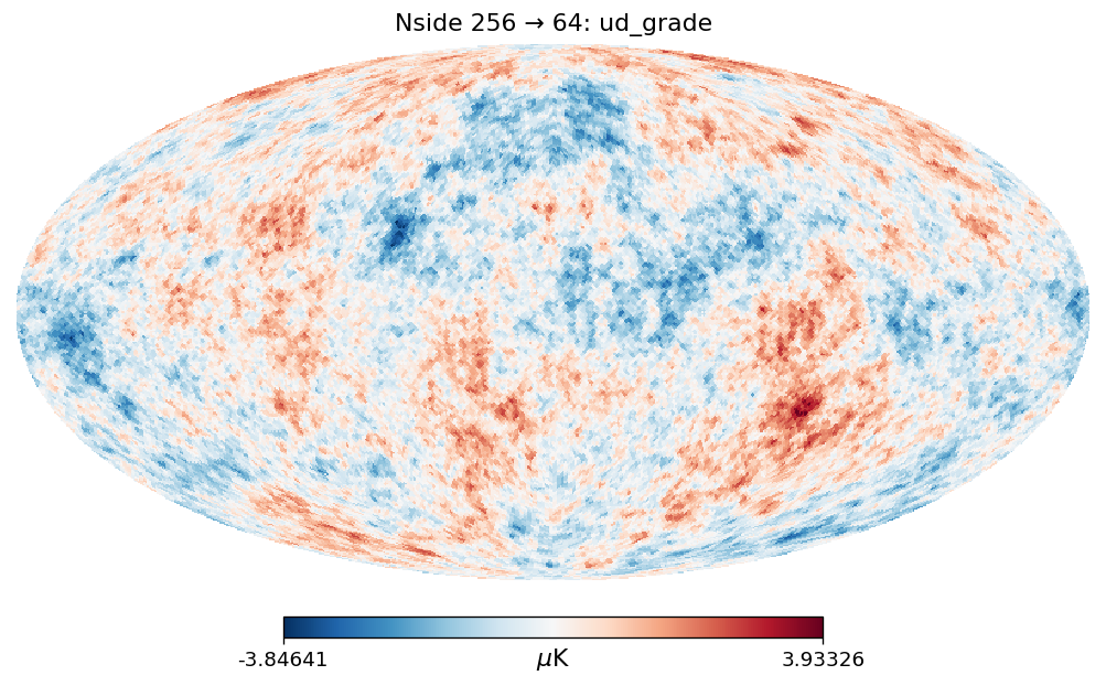
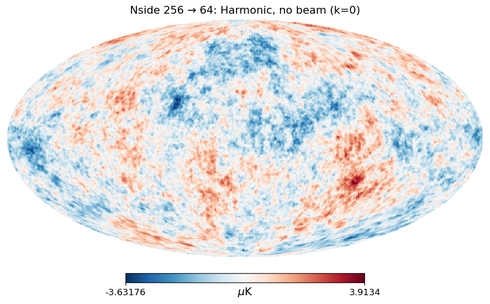
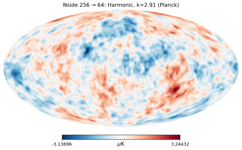
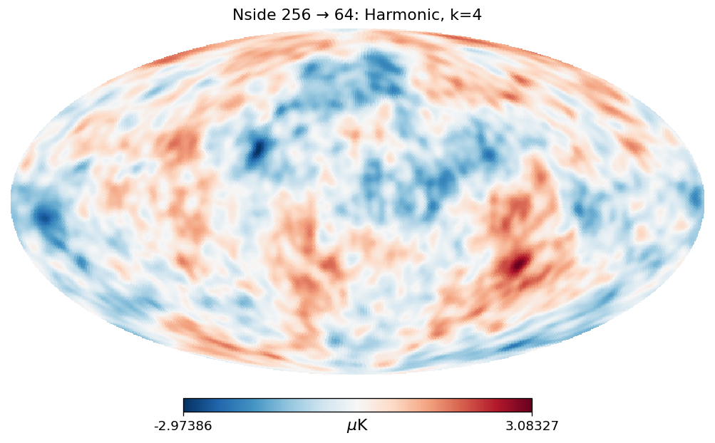
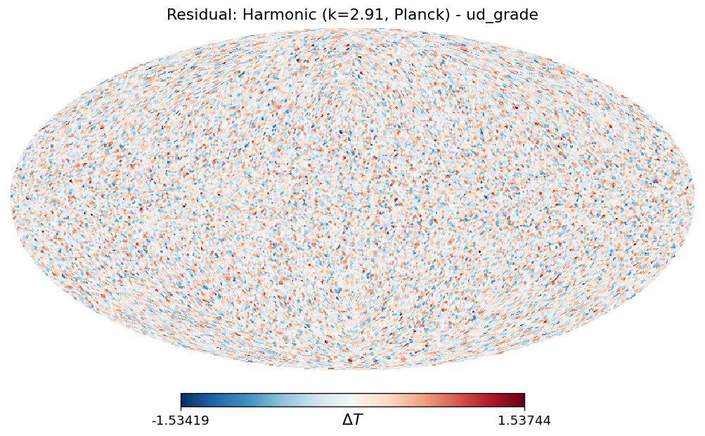
Let’s look at the maps themselves. We visually compare four downgraded maps — ud_grade, harmonic with no beam (\(k=0\)), \(k=3\), and \(k=4\) — and then quantify the pixel-by-pixel difference between the harmonic \(k=3\) map and ud_grade to show that the two approaches are not equivalent.
# Visual comparison of downgraded mapstitles = ["ud_grade","Harmonic, no beam (k=0)",f"Harmonic, k={PLANCK_K:.2f} (Planck)","Harmonic, k=4",]maps_to_show = [map_ud, results[0], results[PLANCK_K], results[4]]for m, title inzip(maps_to_show, titles): hp.mollview(m, title=f"Nside {nside_in} → {nside_out}: {title}", cmap="RdBu_r", unit=r"$\mu$K") plt.show()
What we see: The Mollweide maps show that all methods reproduce the large-scale structure faithfully — differences are concentrated at the pixel scale, as expected since anti-aliasing primarily affects the highest multipoles. The \(k=0\) map retains the sharpest small-scale features (no smoothing), while \(k=4\) is visibly the smoothest.
The residual map (harmonic \(k=2.91\) Planck minus ud_grade) isolates the difference between the two approaches. It is dominated by small-scale structure, confirming that ud_grade and the harmonic method diverge mainly at the pixel scale. The residual RMS is a large fraction of the map RMS — the two methods are not interchangeable. The harmonic approach with pixel-window correction and the Planck beam is more faithful to the true underlying spectrum, while ud_grade introduces a systematic suppression of high-\(\ell\) power through pixel-window aliasing and the absence of a correction transfer function.
10. Summary and Takeaways
Why ~2.91 pixels per beam (colloquially “3”)?
Reason
Detail
Anti-aliasing
At \(k=2.91\), the Gaussian beam amplitude at the HEALPix bandlimit \(\ell_{\max} = 3 N_{\mathrm{side}}-1\) is \(\approx 0.00075\) — >99.9% suppression — preventing aliasing from power near the Nyquist-like rate.
Combined with pixel window
The product \(b_\ell \cdot p_\ell\) at \(k=2.91\) is \(\approx 5 \times 10^{-4}\) at \(\ell_{\max}\), essentially eliminating all aliasing from near-bandlimit power.
Information preservation
\(k=2.91\) preserves the beam transfer function above 50% out to \(\ell \approx 0.30 \times \ell_{\max}\) — a useful fraction of the resolvable bandwidth. \(k=4\) pushes this down to only 22%, unnecessarily discarding information.
Practical tradition
The ~3-pixel convention has roots in radio/optical astronomy sampling theory (Robertson 2017) and was codified for CMB analysis by Planck (2013 XXIII, 2015 XVI) at the precise ratio of 2.91.
Exact Planck prescription
Planck uses FWHM = 160 arcmin × (64 / Nside) across all resolutions (Table 1, Planck 2013 XXIII), which yields a constant FWHM/pixel ratio of 2.91 — not exactly 3. The “3 pixels per beam” label is a convenient approximation. In code:
No.Sullivan, Hergt & Scott (2024) state explicitly that the factor of ~3 is “just a guideline, not a rule.” There is no single theorem that derives it. It is a practical compromise between aliasing suppression and resolution preservation, empirically validated across Planck analyses. The transition from “insufficient” (\(k=2\): 3% amplitude at bandlimit) to “near-perfect” (\(k=2.91\): <0.1%) suppression is steep — the ~3 regime is where the law of diminishing returns sets in.
When to deviate
Point sources / compact bright regions: Band-limiting causes Gibbs ringing. A larger beam (\(k=4\) or more) may be needed, or a pixel-space approach may be preferable.
High signal-to-noise, well-characterized noise: Smaller \(k\) preserves more resolution; the aliasing bias may be acceptable or correctable.
Mask degradation: Planck uses exactly \(k=2.91\); for smooth masks this is well-tested.