GNILC dust zero-level offset with the Lenz et al. 2017 low-velocity HI map
The original measurement of the zero-level offset of the GNILC F353 dust input used the full HI4PI column density map, which includes all gas within |v_LSR| < 600 km/s: high-velocity clouds contribute column density but essentially no dust, biasing the N_HI-FIR correlation. Following the feedback from @ginleaf on PySM issue #281, this notebook redoes the measurement with the Lenz et al. 2017 low-velocity map, |v_LSR| < 90 km/s. The bias on the intercept turns out to be only +0.0011 MJy/sr: the offset is confirmed at +0.1265 MJy/sr, and the templates regenerated with +0.1254 MJy/sr remain valid well within the systematic uncertainties.
Why this notebook
The original measurement of the zero-level offset of the GNILC F353 dust input used the HI4PI column density map, which includes all HI gas within |v_LSR| < 600 km/s. As @ginleaf pointed out in PySM issue #281, high-velocity clouds carry little or no dust, so including them biases the N_HI-FIR correlation and the recovered isotropic term.
The proposed fix is the Lenz et al. 2017 column density map, which only includes low-velocity gas, |v_LSR| < 90 km/s. This notebook redoes the measurement with that map and quantifies the difference between the two tracers.
Method
Same as the original analysis: regressed against outside the GAL080 mask (the mask used by the preprocessing pipeline), on diffuse lines of sight (), both maps smoothed to a common 80 arcmin beam at NSIDE 512, with iterative 3-sigma clipping and a bootstrap for the statistical uncertainty. The fit is repeated with both HI maps, treated identically.
Run on an HPC compute node through Slurm; input locations come from environment
variables (PYSM_DATA, HI4PI_FILENAME, HI4PI_LOWV_FILENAME).
import os
from pathlib import Path

import healpy as hp
import matplotlib.pyplot as plt
import numpy as np
from astropy import units as u
from astropy.table import Table

PYSM_DATA = Path(os.environ.get("PYSM_DATA", "pysm-data"))
GNILC_I353_FILENAME = PYSM_DATA / "dust_gnilc/inputs/COM_CompMap_Dust-GNILC-F353_2048_21p8acm.fits"
GAL080_MASK_FILENAME = PYSM_DATA / "dust_gnilc/raw/HFI_Mask_GalPlane-apo2_2048_R2.00_GAL080_noapo.fits.gz"
HI4PI_FILENAME = Path(os.environ.get("HI4PI_FILENAME", "NHI_HPX.fits"))
HI4PI_LOWV_FILENAME = Path(os.environ.get("HI4PI_LOWV_FILENAME", "mom0_-90_90_1024.hpx.fits"))

NSIDE_ANALYSIS = 512
FWHM_ARCMIN = 80.0
NHI_MAX = 3.0
NSIGMA_CLIP = 3.0
N_BOOTSTRAP = 200

print("numpy", np.__version__, "| healpy", hp.__version__)
print("GNILC I353  :", GNILC_I353_FILENAME)
print("GAL080 mask :", GAL080_MASK_FILENAME)
print("HI4PI full  :", HI4PI_FILENAME)
print("HI4PI low-v :", HI4PI_LOWV_FILENAME)
numpy 2.4.6 | healpy 1.20.1
GNILC I353 : ~/issue_281/pysm-data/dust_gnilc/inputs/COM_CompMap_Dust-GNILC-F353_2048_21p8acm.fits
GAL080 mask : ~/issue_281/pysm-data/dust_gnilc/raw/HFI_Mask_GalPlane-apo2_2048_R2.00_GAL080_noapo.fits.gz
HI4PI full : ~/issue_281/data/NHI_HPX.fits
HI4PI low-v : ~/issue_281/data/mom0_-90_90_1024.hpx.fitsLoad the maps
- GNILC F353, 21.8’ beam: the intensity input of the d9/d10/d11 preprocessing, in MJy/sr.
- HI4PI N_HI: full column density, |v_LSR| < 600 km/s; a binary table with
explicit
HPXINDEXandNHIcolumns. - Lenz et al. 2017 N_HI: low-velocity column density, |v_LSR| < 90 km/s; a
binary table with a single
NHIcolumn in HEALPix RING pixel order.
i353_2048 = hp.read_map(GNILC_I353_FILENAME, dtype=np.float64)
gal080_2048 = hp.read_map(GAL080_MASK_FILENAME, dtype=np.float64)

# full HI4PI column density, explicit pixel indices
hi4pi_table = Table.read(HI4PI_FILENAME, hdu=1)
nhi_full_1024 = np.full(hp.nside2npix(1024), np.nan)
nhi_full_1024[hi4pi_table["HPXINDEX"].astype(int)] = hi4pi_table["NHI"]

# Lenz et al. 2017 low-velocity column density, single column in RING order
nhi_lowv_1024 = np.array(Table.read(HI4PI_LOWV_FILENAME, hdu=1)["NHI"], dtype=np.float64)

print("full HI4PI missing pixels:", int(np.isnan(nhi_full_1024).sum()))
print(f"N_HI full   : {np.nanmin(nhi_full_1024):.2e} to {np.nanmax(nhi_full_1024):.2e} cm^-2")
print(f"N_HI |v|<90 : {nhi_lowv_1024.min():.2e} to {nhi_lowv_1024.max():.2e} cm^-2")
full HI4PI missing pixels: 0
N_HI full : -1.60e+21 to 2.40e+22 cm^-2
N_HI |v|<90 : -1.68e+21 to 2.03e+22 cm^-2fwhm = np.radians(FWHM_ARCMIN / 60.0)
i353 = hp.ud_grade(hp.smoothing(i353_2048, fwhm=fwhm), nside_out=NSIDE_ANALYSIS)
del i353_2048
nhi_full = hp.ud_grade(hp.smoothing(nhi_full_1024, fwhm=fwhm), nside_out=NSIDE_ANALYSIS) / 1e20
nhi_lowv = hp.ud_grade(hp.smoothing(nhi_lowv_1024, fwhm=fwhm), nside_out=NSIDE_ANALYSIS) / 1e20
del nhi_full_1024, nhi_lowv_1024
outside_plane = hp.ud_grade(gal080_2048, nside_out=NSIDE_ANALYSIS) > 0.5
del gal080_2048
print(f"outside GAL080: {outside_plane.sum():,} pixels "
f"({100 * outside_plane.mean():.2f}% of the sky)")outside GAL080: 2,488,934 pixels (79.12% of the sky)plt.figure(figsize=(18, 5))
hp.mollview(nhi_full, sub=(1, 3, 1), title="HI4PI N_HI, |v| < 600 km/s",
unit=r"$10^{20}$ cm$^{-2}$", norm="hist")
hp.mollview(nhi_lowv, sub=(1, 3, 2), title="Lenz et al. 2017 N_HI, |v| < 90 km/s",
unit=r"$10^{20}$ cm$^{-2}$", norm="hist")
hp.mollview(nhi_full - nhi_lowv, sub=(1, 3, 3),
title="intermediate and high velocity gas (the difference)",
unit=r"$10^{20}$ cm$^{-2}$")
plt.show()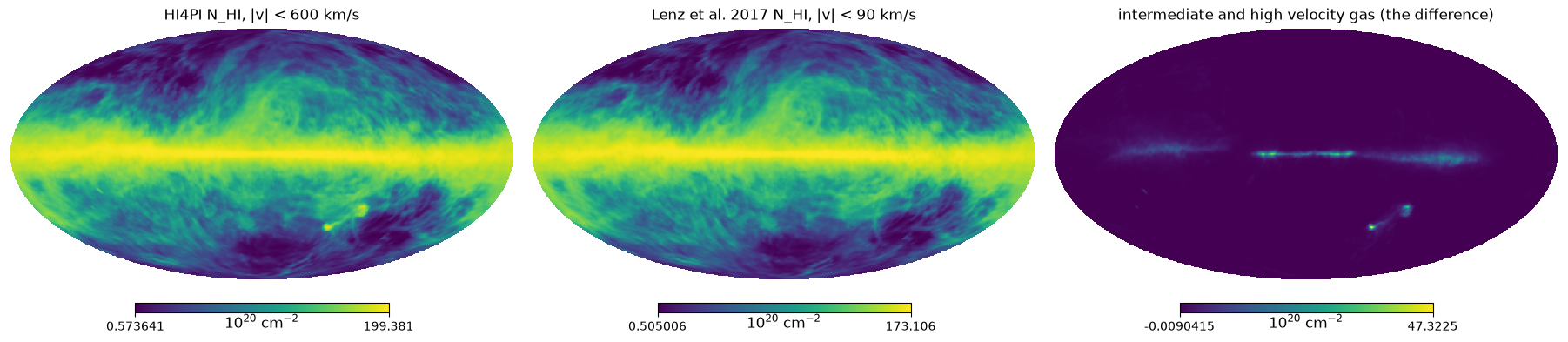
Robust linear fit, with both tracers
with iterative 3-sigma clipping; the bootstrap gives the statistical error on slope and intercept (correlated pixels still make it an underestimate, the N_HI cuts below give the systematic scale). The same selection and the same procedure are applied to both HI maps, so the difference between the two intercepts is the bias introduced by the intermediate and high velocity gas.
def robust_linear_fit(x, y, nsigma=NSIGMA_CLIP, n_iter=6):
    keep = np.ones(len(x), dtype=bool)
    for _ in range(n_iter):
        slope, intercept = np.polyfit(x[keep], y[keep], 1)
        residual = y - (slope * x + intercept)
        sigma = np.std(residual[keep])
        keep = np.abs(residual) < nsigma * sigma
    return slope, intercept, keep


fits = {}
for label, nhi in [("full HI4PI (|v|<600)", nhi_full),
                   ("low-velocity (|v|<90)", nhi_lowv)]:
    selection = outside_plane & (nhi < NHI_MAX) & np.isfinite(i353) & np.isfinite(nhi)
    x, y = nhi[selection], i353[selection]
    slope, intercept, keep = robust_linear_fit(x, y)
    rng = np.random.default_rng(12345)
    xf, yf = x[keep], y[keep]
    slopes_boot = np.empty(N_BOOTSTRAP)
    intercepts_boot = np.empty(N_BOOTSTRAP)
    for i in range(N_BOOTSTRAP):
        idx = rng.integers(0, len(xf), len(xf))
        slopes_boot[i], intercepts_boot[i] = np.polyfit(xf[idx], yf[idx], 1)
    fits[label] = {
        "slope": float(slope),
        "intercept": float(intercept),
        "intercept_err": float(intercepts_boot.std()),
        "n": int(selection.sum()),
        "n_keep": int(keep.sum()),
        "selection": selection,
        "keep": keep,
    }
    print(f"{label}: {selection.sum():,} pixels selected, "
          f"{keep.sum():,} after clipping")
    print(f"  slope    : {slope:.4f} +/- {slopes_boot.std():.4f}"
          f" MJy/sr per 1e20 cm^-2")
    print(f"  intercept: {intercept:+.4f} +/- {intercepts_boot.std():.4f} MJy/sr")

bias = (fits["low-velocity (|v|<90)"]["intercept"]
        - fits["full HI4PI (|v|<600)"]["intercept"])
print(f"\nintercept difference (low-velocity minus full HI4PI): {bias:+.4f} MJy/sr")
full HI4PI (|v|<600): 884,242 pixels selected, 857,201 after clipping
slope : 0.0377 +/- 0.0000 MJy/sr per 1e20 cm^-2
intercept: +0.1254 +/- 0.0000 MJy/srlow-velocity (|v|<90): 911,059 pixels selected, 886,027 after clipping
slope : 0.0387 +/- 0.0000 MJy/sr per 1e20 cm^-2
intercept: +0.1265 +/- 0.0000 MJy/sr
intercept difference (low-velocity minus full HI4PI): +0.0011 MJy/srfit_lv = fits["low-velocity (|v|<90)"]
selection, keep = fit_lv["selection"], fit_lv["keep"]
x, y = nhi_lowv[selection], i353[selection]
xf, yf = x[keep], y[keep]
fig, ax = plt.subplots(figsize=(11, 7))
hb = ax.hexbin(xf, yf, gridsize=250, bins="log", cmap="viridis", mincnt=1)
fig.colorbar(hb, ax=ax, label="log10(count per hexagon)")
nbins = 15
bins = np.linspace(xf.min(), xf.max(), nbins + 1)
centers = 0.5 * (bins[:-1] + bins[1:])
means = np.array([yf[(xf >= bins[i]) & (xf < bins[i + 1])].mean() for i in range(nbins)])
ax.plot(centers, means, "o-", color="crimson", lw=2, label="binned mean")
xx = np.linspace(0, xf.max(), 10)
ax.plot(xx, fit_lv["slope"] * xx + fit_lv["intercept"], "-", color="orange", lw=2,
label="fit: I = %.3f N_HI %+.3f" % (fit_lv["slope"], fit_lv["intercept"]))
ax.axhline(0.0, color="gray", ls=":", lw=1)
ax.set_xlabel(r"$N_{HI}$ (|v| < 90 km/s) [$10^{20}$ cm$^{-2}$]")
ax.set_ylabel(r"$I_{353}$ [MJy/sr]")
ax.set_title("GNILC I_353 vs low-velocity N_HI (80' beam, outside GAL080, 3-sigma clipped)")
ax.legend()
plt.show()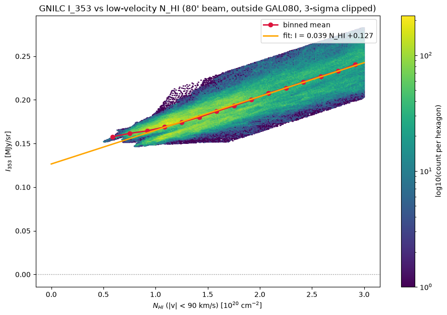
fit_full = fits["full HI4PI (|v|<600)"]
residual_lv = i353 - fit_lv["slope"] * nhi_lowv

sel_lv, keep_lv = fit_lv["selection"], fit_lv["keep"]
keep_sky = np.zeros(i353.size, dtype=bool)
keep_sky[np.where(sel_lv)[0][keep_lv]] = True

plt.figure(figsize=(10, 6))
plt.hist(residual_lv[keep_sky], bins=200, density=True, color="steelblue", alpha=0.8)
plt.axvline(fit_lv["intercept"], color="orange", lw=2,
            label="low-velocity intercept = %+.4f MJy/sr" % fit_lv["intercept"])
plt.axvline(fit_full["intercept"], color="purple", lw=2, ls="--",
            label="full HI4PI intercept = %+.4f MJy/sr" % fit_full["intercept"])
plt.axvline(0.13, color="red", ls=":", lw=2, label="0.13 MJy/sr (Planck 2018 XII)")
plt.xlabel(r"$I_{353} - \epsilon\ N_{HI}$ [MJy/sr]")
plt.ylabel("pixels (density)")
plt.legend()
plt.show()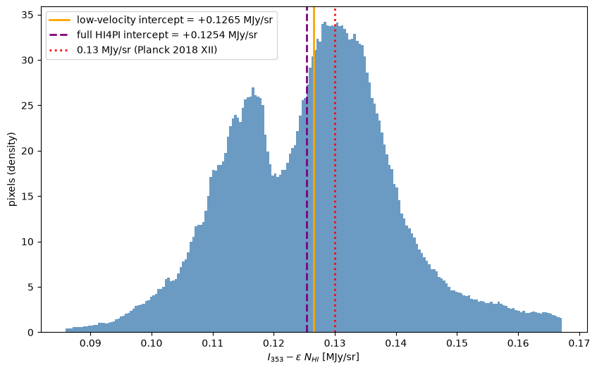
theta, phi = hp.pix2ang(NSIDE_ANALYSIS, np.arange(hp.nside2npix(NSIDE_ANALYSIS)))
glat = 90.0 - np.degrees(theta)

print(f"{'selection':>28} {'pixels':>12} {'slope':>8} {'intercept':>10}")
for nhi_max in [2.0, 3.0, 4.0, 5.0]:
    sel_k = outside_plane & (nhi_lowv < nhi_max) & np.isfinite(i353)
    s, b, k = robust_linear_fit(nhi_lowv[sel_k], i353[sel_k])
    print(f"{'outside GAL080, N_HI < %.0fe20' % nhi_max:>28} {int(k.sum()):>12,} "
          f"{s:>8.4f} {b:>+10.4f}")
for nhi_max in [2.0, 3.0]:
    sel_k = (np.abs(glat) > 30.0) & (nhi_lowv < nhi_max) & np.isfinite(i353)
    s, b, k = robust_linear_fit(nhi_lowv[sel_k], i353[sel_k])
    print(f"{'|b| > 30 deg, N_HI < %.0fe20' % nhi_max:>28} {int(k.sum()):>12,} "
          f"{s:>8.4f} {b:>+10.4f}")
selection pixels slope intercept outside GAL080, N_HI < 2e20 569,350 0.0349 +0.1314 outside GAL080, N_HI < 3e20 886,027 0.0387 +0.1265 outside GAL080, N_HI < 4e20 1,193,823 0.0422 +0.1211 outside GAL080, N_HI < 5e20 1,465,991 0.0445 +0.1172 |b| > 30 deg, N_HI < 2e20 568,548 0.0348 +0.1314 |b| > 30 deg, N_HI < 3e20 858,959 0.0380 +0.1274Why does removing the high-velocity gas raise the intercept?
At first sight, less gas in the tracer should leave less for the intercept. But dust-free column density affects the regression in two competing ways, both of order a few 0.001 MJy/sr, which almost cancel:
- It dilutes the slope. The high-velocity column is uncorrelated with the dust emission, so it acts as noise on the x axis: the fitted slope is attenuated (errors-in-variables), 0.0387 -> 0.0373 here. A flatter line explains less of the mean dust emission per unit column, and what is left over flows into the intercept: this pushes the intercept up, by .
- It absorbs emission into the correlated term. The mean high-velocity column, about 5% of the dust column, is still multiplied by the positive fitted slope, so the fit attributes about of emission to correlated dust that is not there: this pushes the intercept down.
Which one wins depends on how patchy the contaminating gas is: the dilution scales with its variance, the absorption with its mean. High-velocity clouds are extremely patchy: over the selected pixels they contribute only a few percent of the mean column but a much larger fraction of the variance. The dilution therefore slightly dominates, and removing the high-velocity gas raises the intercept.
The cell below measures both terms on the same pixel selection (chosen with the clean tracer), so the two fits differ only through the tracer, not through the selected pixels.
# Fit both tracers on the SAME pixels, so the difference isolates the effect of
# the tracer from the effect of the selection.
nhi_hvc = nhi_full - nhi_lowv
sel_same = outside_plane & (nhi_lowv < NHI_MAX) & np.isfinite(i353)

b_d, a_d, keep_d = robust_linear_fit(nhi_lowv[sel_same], i353[sel_same])
b_f, a_f, keep_f = robust_linear_fit(nhi_full[sel_same], i353[sel_same])
print(f"clean tracer: slope {b_d:.4f}  intercept {a_d:+.4f} MJy/sr")
print(f"full tracer : slope {b_f:.4f}  intercept {a_f:+.4f} MJy/sr")
print(f"intercept difference on the same pixels: {a_d - a_f:+.4f} MJy/sr")

x_d = nhi_lowv[sel_same][keep_d]
x_h = nhi_hvc[sel_same][keep_d]
x_f = nhi_full[sel_same][keep_d]
print(f"\nmeans (1e20 cm^-2): dust {x_d.mean():.3f}  high-velocity {x_h.mean():.4f}")
print(f"vars  (1e20^2):     dust {x_d.var():.3f}  high-velocity {x_h.var():.4f}  full {x_f.var():.3f}")
print(f"CV (std/mean):      dust {np.sqrt(x_d.var()) / x_d.mean():.2f}  "
      f"high-velocity {np.sqrt(x_h.var()) / max(x_h.mean(), 1e-9):.2f}")

print(f"\nslope-dilution term  (eps-b)*<N_dust> = {+(b_d - b_f) * x_d.mean():+.4f} MJy/sr  [intercept UP]")
print(f"absorption term      -b*<N_hvc>       = {-b_f * x_h.mean():+.4f} MJy/sr  [intercept DOWN]")
clean tracer: slope 0.0387 intercept +0.1265 MJy/sr
full tracer : slope 0.0373 intercept +0.1261 MJy/sr
intercept difference on the same pixels: +0.0004 MJy/sr
means (1e20 cm^-2): dust 1.788 high-velocity 0.0898
vars (1e20^2): dust 0.362 high-velocity 0.0686 full 0.445
CV (std/mean): dust 0.34 high-velocity 2.92
slope-dilution term (eps-b)*<N_dust> = +0.0024 MJy/sr [intercept UP]
absorption term -b*<N_hvc> = -0.0034 MJy/sr [intercept DOWN]Reading the results
The intercept measured with the low-velocity HI map is the updated estimate of the isotropic offset of the GNILC F353 input map (CIB monopole + residual zodiacal emission + any zero-level offset of the GNILC processing). The difference with the original, full-HI4PI measurement is the bias introduced by the intermediate and high velocity gas that @ginleaf flagged: gas which contributes column density but essentially no dust emission, diluting the correlation and shifting the intercept.
Measured with the same procedure, the low-velocity intercept is +0.1265 MJy/sr against +0.1254 MJy/sr for the full map: the bias introduced by the intermediate and high velocity gas is only +0.0011 MJy/sr, an order of magnitude below the ~0.01 MJy/sr systematic scale set by the N_HI cuts. The dust emissivity slope increases slightly, from 0.0377 to 0.0387 MJy/sr per 1e20 cm^-2, as expected when dust-free column density is removed from the tracer.
The conclusions of the original analysis are unchanged in their essentials: the offset is close to the 0.13 MJy/sr that the preprocessing intended to subtract, and the regenerated templates (see the original post and the issue for the details) remain valid within these systematic uncertainties.
Caveats, as before: molecular and ionized gas are not traced by N_HI and partly end up in the intercept, the choice of the N_HI cut matters at the ~0.01 MJy/sr level, and the velocity cut of the HI tracer is itself a systematic, as this notebook shows.
import json

results = {
    "full_hi4pi": {k: fits["full HI4PI (|v|<600)"][k]
                   for k in ["slope", "intercept", "intercept_err", "n", "n_keep"]},
    "low_velocity_lenz2017": {k: fits["low-velocity (|v|<90)"][k]
                              for k in ["slope", "intercept", "intercept_err", "n", "n_keep"]},
    "hvc_intercept_bias": float(bias),
    "nhi_max_1e20": NHI_MAX,
    "fwhm_arcmin": FWHM_ARCMIN,
    "nside": NSIDE_ANALYSIS,
}
with open("gnilc_dust_offset_lowvel_results.json", "w") as f:
    json.dump(results, f, indent=2)
print(json.dumps(results, indent=2))
{
"full_hi4pi": {
"slope": 0.0377347503478262,
"intercept": 0.1254091430985887,
"intercept_err": 4.882632225954523e-05,
"n": 884242,
"n_keep": 857201
},
"low_velocity_lenz2017": {
"slope": 0.03867443356936235,
"intercept": 0.12654373866151822,
"intercept_err": 4.270933811138979e-05,
"n": 911059,
"n_keep": 886027
},
"hvc_intercept_bias": 0.0011345955629295246,
"nhi_max_1e20": 3.0,
"fwhm_arcmin": 80.0,
"nside": 512
}